Model Evaluation
This describes how to evaluate an ML model using the MLTK model evaluation command/API.
Note
This document focuses on the evaluation aspect of model development. Refer to the tutorials for end-to-end guides on how to develop an ML model.
Quick Reference
Command-line: mltk evaluate –help
Python API: evaluate_model
Python API examples: evaluate_model.ipynb
Overview
Model evaluation involves running test samples (i.e. new samples, not used for model training) through the trained model and comparing the trained model’s output versus the expected output.
The basic sequence for using the MLTK’s evaluation feature is:
Add an evaluation “mixin” to the model specification script
Train the model
Invoke model evaluation using the Command-line or Python API
When evaluation completes, the model archive file is updated with the evaluation results. The evaluation results indicate how well the model might perform with real data.
Non-Quantized vs Quantized Model Evaluation
Two model files are generated at the end of training:
Keras Model - This is the non-quantized, actual model that was trained using float32 weights, file extension:
.h5Tensorflow-Lite Model - This is the converted, quantized model with int8 weights that can execute on an embedded device, file extension:
.tflite(see Model Quantization)
Both these models should produce similar results, however, the .tflite model may be ~1-5% less accuracy than the .h5 due to the quantization (i.e. compression) of its weights.
By default, the evaluate command or evaluate_model API will use the .h5 model for evaluation.
Specify the --tflite option to evaluate using the .tflite (i.e. quantized) model.
Model Profiling vs Model Evaluation
It is important to note the difference between model profiling and model evaluation:
Model Profiling - Measure how efficiently a model executes (i.e. time & energy)
Model Evaluation - Measure how well a model is able to make predictions (i.e. accuracy)
Model Specification
All model parameters are defined in the Model Specification script. This is a standard Python script that defines a MltkModel instance.
To enable evaluation, the MltkModel instance must inherit an evaluation “mixin” such as:
EvaluateMixin - Generic evaluation for custom models
EvaluateClassifierMixin - Evaluate a classification model
EvaluateAutoEncoderMixin - Evaluate an auto-encoder model
For example, the following might be added to the top of my_model_v1.py:
# Define a new MyModel class which inherits the
# MltkModel and several mixins
# @mltk_model
class MyModel(
    MltkModel,
    TrainMixin,
    AudioDatasetMixin,
    EvaluateClassifierMixin
):
    """My Model's class object"""

# Instantiate the MyModel class
my_model = MyModel()
Here we define our model’s class object: MyModel.
Among other mixins, this custom class inherits EvaluateClassifierMixin which enables the MLTK’s evaluation feature with this classification model.
See the Model Specification documentation for more details.
Evaluation Results
The results generated by model evaluation are specific to the evaluation “mixin” used in the model specification:
EvaluateClassifierMixin - Generate “classifier” specific evaluation results
EvaluateAutoEncoderMixin - Generate “auto encoder” specific evaluation results
EvaluateMixin - Generate custom evaluation results
EvaluateClassifierMixin
The EvaluateClassifierMixin is specific to “Classifier” models.
It returns a ClassifierEvaluationResults object.
The following diagrams are generated by this mixin:
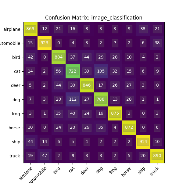
Confusion Matrix
A specific table layout that allows visualization of the performance of an algorithm. Each row of the matrix represents the instances in an actual class while each column represents the instances in a predicted class, or vice versa. See Confusion Matrix for more details.
Example:
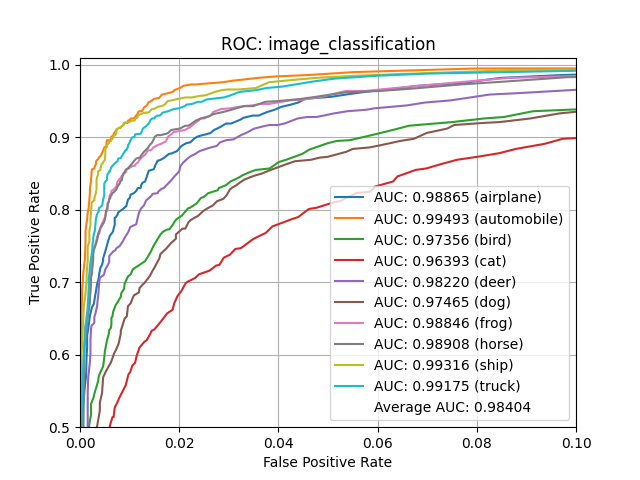
ROC
A receiver operating characteristic curve, or ROC curve, is a graphical plot that illustrates the diagnostic ability of a binary classifier system as its discrimination threshold is varied. The ROC curve is created by plotting the true positive rate (TPR) against the false positive rate (FPR) at various threshold settings. See Receiver Operating Characteristic for more details.
Example:
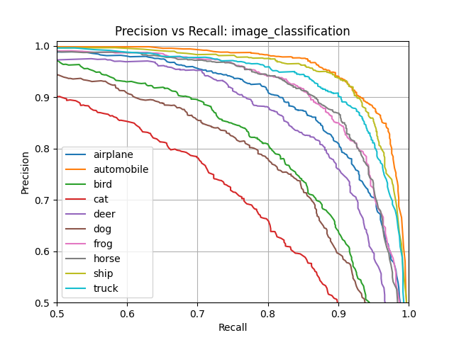
Precision vs Recall
Precision (also called positive predictive value) is the fraction of relevant instances among the retrieved instances, while recall (also known as sensitivity) is the fraction of relevant instances that were retrieved. See Precision and Recall for more details.
Example:
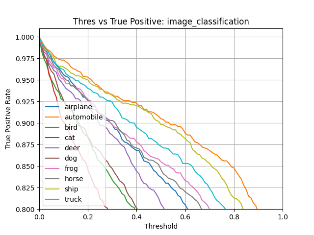
True Positive Rate
True Positive Rate refers to the proportion of those who have the condition (when judged by the ‘Gold Standard’) that received a positive result on this test. See True Positive Rate for more details.
Example:
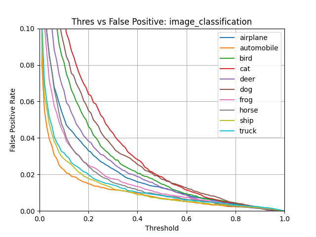
False Positive Rate
In statistics, when performing multiple comparisons, a false positive ratio (also known as fall-out or false alarm ratio) is the probability of falsely rejecting the null hypothesis for a particular test. The false positive rate is calculated as the ratio between the number of negative events wrongly categorized as positive (false positives) and the total number of actual negative events (regardless of classification). See False Positive Rate for more details.
Example:
EvaluateAutoEncoderMixin
The EvaluateAutoEncoderMixin is specific to “Auto Encoder” models.
It returns a AutoEncoderEvaluationResults object.
Command
Model evaluation from the command-line is done using the evaluate operation.
For more details on the available command-line options, issue the command:
mltk evaluate --help
The following are examples of how evaluation can be invoked from the command-line:
Example 1: Evaluate Classification .h5 Model
The following example evaluates the image_example1 model
using the .h5 (i.e. non-quantized, float32 weights) model file.
This is a “classification” model, i.e. given an input, the model predicts to which
“class” the input belongs.
The model archive is updated with the evaluation results.
Additionally, the --show option displays interactive diagrams.
mltk evaluate image_example1 --show
Example 2: Evaluate Classification .tflite Model
The following example evaluates the image_example1 model
using the .tflite (i.e. quantized, int8 weights) model file.
This is a “classification” model, i.e. given an input, the model predicts to which
“class” the input belongs.
The model archive is updated with the evaluation results.
Additionally, the --show option displays interactive diagrams.
mltk evaluate image_example1 --tflite --show
Example 3: Evaluate Auto-Encoder .h5 Model
The following example evaluates the anomaly_detection model
using the .h5 (i.e. non-quantized, float32 weights) model file.
This is an “auto-encoder” model, i.e. given an input, the model attempts to reconstruct
the same input. The worse the reconstruction, the further the input is from what the
model was trained against, this indicates that an anomaly may be detected.
The model archive is updated with the evaluation results.
Additionally, the --show option displays interactive diagrams and the --dump
option dumps a comparison image between the input and reconstructed image.
mltk evaluate anomaly_detection --show --dump
Python API
Model evaluation is accessible via evaluate_model API.
Examples using this API may be found in evaluate_model.ipynb