Keyword Spotting Overview
An overview of how to detect keywords using Machine Learning (ML) on an embedded device
What is Keyword Spotting?
The basic idea behind keyword spotting is a machine learning (ML) model is trained to detect specific words, e.g. "On", "Off". On an embedded device, microphone audio is fed into the ML model, and if it detects a word it notifies the firmware application which reacts accordingly.
ML Model
Notify firmware application

How is it implemented?
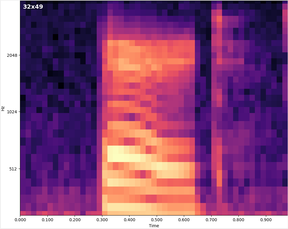
- Convert audio to spectrogram image
- Run spectrogram image through CNN ML model
- The output of ML model is the probability of each possible keyword being seen in the spectrogram
- Optionally, execute steps 1-3 multiple times to gain a running average of each keywords' probability. If a given keyword's average probability is greater than a threshold, then the keyword is considered detected
Data Flow

1) Capture microphone audio
2) Convert audio into 2D spectrogram image
Machine Learning
Model
3) Provide spectrogram image to ML Model.
The output of the ML model is the probability of each possible keyword being in the spectrogram, e.g:
On: 95%, Off: 4%, Silence: 0.3%, Unknown: 0.7%
IF MAX(averaged_predictions) > threshold:
   keyword_id = ARGMAX(averaged_predictions)
   notify_application(keyword_id)
Optionally, repeat step 1-3 multiple times and calculate a running average of each keywords' probability
4) If the probability of a given keyword exceeds a threshold, then the keyword is considered detected. Notify the application.
Note About Latency
- For a keyword to be detected, it needs to be "seen" multiple times by the ML model for its average probability to exceed the threshold
- This means the processing time directly affects the embedded device's ability to detect keywords
- In other words, the longer it takes the device to process the audio sample, e.g. <Spectrogram Generation Time> + <ML Inference Time>, the fewer times a keyword is processed which reduces the averaging and thus keyword detection confidence
Fast Processing
The following video shows a 1s audio sample being processed in increments of 100ms. So the ML model "sees" the same audio sample shifted by 100ms. 100ms is the simulated amount of time it takes the embedded device to generate the spectrogram and process it in the ML model. In this case, there are many predictions in the running average giving high confidence of a keyword detection.
NOTE: This video was created using the view_audio MLTK command
Slow Processing
The following video shows a 1s audio sample being processed in increments of 400ms. So the ML model "sees" the same audio sample shifted by 400ms. 400ms is the simulated amount of time it takes the embedded device to generate the spectrogram and process it in the ML model. In this case, there are few predictions in the running average giving low confidence of a keyword detection.
The video is playing in a loop. In reality, the embedded device would only "see" the audio 2 times
How to Reduce Processing Time?
The following are typical approaches to reducing processing time:
- Decrease the size of the spectrogram
- Decreasing the size of the spectrogram decreases the size of the ML model input which reduces the amount of processing required by the ML model
- Reduce the size of the ML model
- Reduce the number of Conv2D filters
- Use DepthwiseConv2D instead of Conv2D
- Reduce the number of layers in the ML model
- Use a hardware accelerator
- Some Silicon Labs MCUs feature the MVP hardware accelerator which can reduce ML model processing time by 2x
- The MLTK features a Model Profiler which indicates the processing time required by the ML model
Additional Reading
- Keyword Spotting Tutorial - End-to-end tutorial describing how to create a "Keyword Spotting" application
- Audio Utilities - Utilities to aid the development of audio-based machine learning models
- AudioFeatureGenerator - Software library to generate spectrograms from streaming audio